This page introduces the image of long-term asset management, concrete management methods, and the effect of time.
If you set a certain expected rate of return, you can simulate the progress according to your asumed investment period.
You don't need a very difficult formula, just set the amount of the goal with the following formula and change the progress to that goal.
The amount of the goal = Principal × (1 + ERR)n
ERR : Expected rate of Return per year
n : Asumed investment period (years)
In reality, the goal is unsettled, and fortune-telling does not always come true.
However, the path to the goal point is complicated, and if the expected rate of return is reasonable, it is possible to reach the amount of asset at goal even if the goal point is not accurate.
Here, we consider asset management with an expected rate of return of 4.3% per year.
Although rough, let's assume that 30 years have passed with the rate of return in following Table 1, with the standard deviation of about 20%.
If the standard deviation is 20%, the probability of price fluctuations within ±20% (within ±1σ range) is 68%, and the probability of larger fluctuations is 32%.
| Years (year) | 1st | 2nd | 3rd | 4th | 5th | 6th | 7th | 8th | 9th | 10th |
| Rate of return | −10% | −35% | 0% | +10% | −10% | +35% | +15% | +35% | +5% | −10% |
| Years (year) | 11th | 12th | 13th | 14th | 15th | 16th | 17th | 18th | 19th | 20th |
| Rate of return | −30% | +5% | +15% | +35% | −5% | +10% | +25% | +15% | +5% | +20% |
| Years (year) | 21th | 22th | 23th | 24th | 25th | 26th | 27th | 28th | 29th | 30th |
| Rate of return | +10% | −25% | +20% | −5% | −5% | 0% | +15% | +20% | +5% | +10% |
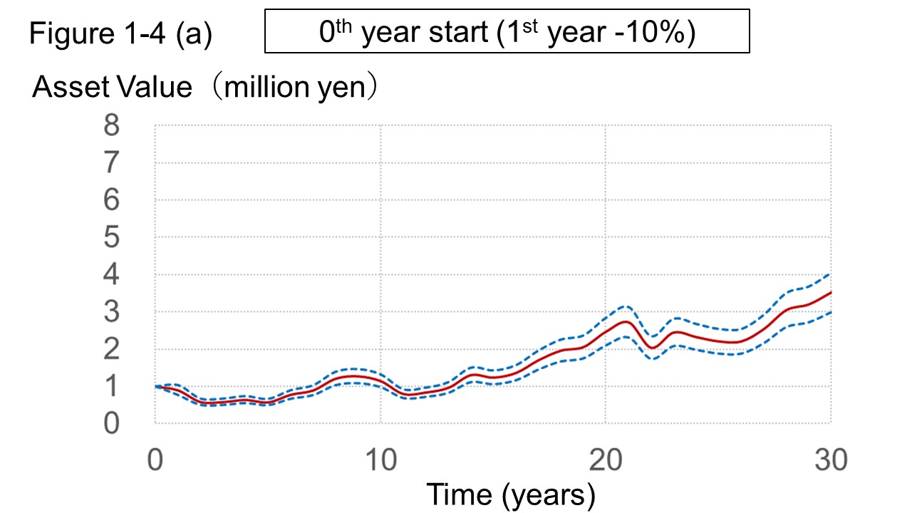
The graph of profit and loss in Table 1 is shown in Figure 1-4 (a) "0th year start".
The blue dotted line shows the range ±15% from the red line and represents the annual change in asset price, which is different from the standard deviation above.
The reason for adding the dotted blue line is to show that it is possible to reach the asset amount of goal due to annual fluctuations even if it is not the assumed timing.
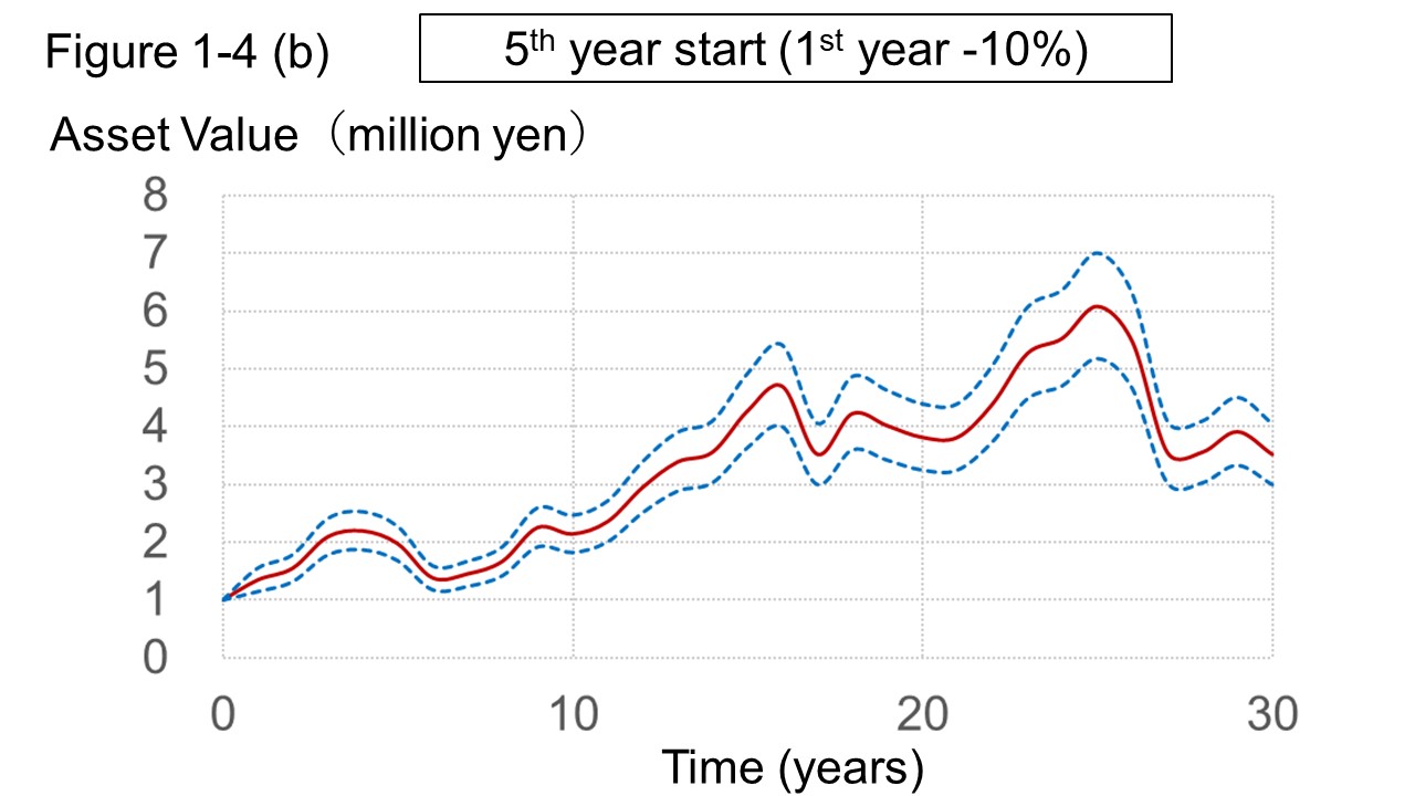
Figure 1-4 (b) "Start in the 5th year" show a graph of the profit and loss when the investing is started from the 5th year and the rate of return before the 5th year is added later.
When the rate of return for the \(n\)th year is represented by \(R_{n}\), the expected rate of return for both the "0th year start" and the "5th year start" is expressed by formula (1).
So in both cases the ultimate goal is the same.
But, the path to the goal is quite different.
The "0th year start" is an unlucky start with a significant loss of assets in the first 5 years.
There was a loss until the 13th year, but after that the return started to become positive at last.
Finally, the asset reached about 3 million yen on an upward trend.
On the other hand, "5th year start" is a lucky start with a significant profit in the first 5 years.
The amount of asset has temporarily reached 6 million yen without loss of the principal in the process.
But, after that, it declined sharply and eventually reached about 3 million yen.
This simulation suggests the following:
- If the expected rate of return is fixed, the value of the asset will eventually reach the same goal, regardless of the path.
- The start timing of investment affects subsequent changes in asset prices.
- Exit timing is as important as start timing.
However, although it is possible for those who can see the timing to invest at the 5th year, it is difficult to see the future 5 years.
In addition to asset diversification, to buy asset at different timings also affects the outcome of your investing.
ref 1
However, there are many ways to buy asset at different timings.
Here, we will consider to buy an asset for a fixed amount or a fixed quantity, limited to regular investing.
The former is called "dollar-cost averaging", which is known that assets can be bought at a lower average price than the latter.
For comparing the two methods, it is inconvenient if the other also does not have a name, so the latter will be called "dollar-quantity accumulating" here.
- dollar-cost averaging
- How to buy an asset for a fixed amount at a regular timing
- dollar-quantity accumulating
- How to buy a certain amount of asset at a regular timing
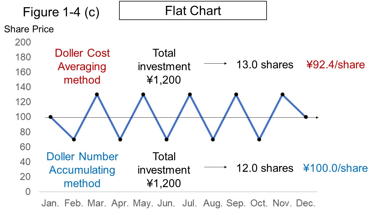
Below, we will consider two case,one is to buy 100 yen worth of shares by the dollar-cost averaging and the other is to buy one share by dollar-quantity accumulating, each month.
Figure 1-4 (c) is a "flat chart" in which the price per share was 100 yen at the beginning and end of the year, and it remained 70 to 130 yen during that period.
In this case, the average acquisition price per share is 92.4 yen in dollar-cost averaging and 100.0 yen in dollar-quantity accumulating, and the dollar-cost averaging show lower acquisition price per share.
However, to reduce the average acquisition price does not always mean that losse will decrease.
Figures 1-4 (d) and 1-4 (e) shown below are charts fliped vertically, which show uptrend and downtrend of stock prices, respectively.
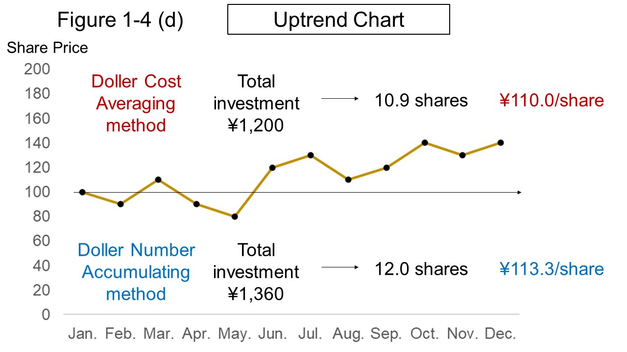
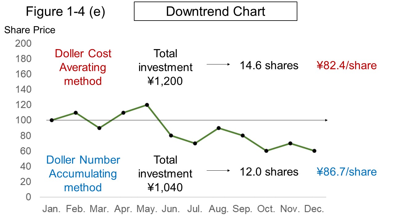
Table 2 shows a comparison of dollar-cost averaging (DCA) and dollar-quantity accumulating (DQA) on these two charts.
The average acquisition price per share is lower in the dollar-cost averaging regardless of the direction of the stock price.
But it can be seen that the loss is the largest in the dollar-cost averaging on downtrend chart.
| Chart/method | Number of shares | Average acquisition price per share | Total investment | Profit and loss | Profit and loss ratio | |
| Uptrend | DCA | 10.9 | 109.8 yen | 1,200 yen | +329 yen | +27.4% |
| DQA | 12.0 | 113.3 yen | 1,360 yen | +320 yen | +23.5% | |
| Downtrend | DCA | 14.6 | 82.4 yen | 1,200 yen | −326 yen | −27.2% |
| DQA | 12.0 | 86.7 yen | 1,040 yen | −320 yen | −30.8% | |
However, there is no problem with the dollar-cost averaging method.
Although doller-cost averaging may increase the "loss amount" when stock prices show downtrend, the "profit and loss ratio" is better than the dollar-quantity accumulating.
Rather, the dollar cost averaging on the downtrend will brings the largest return when the positive expected value is realized because the number of shares held is the most and the average acquisition unit price is the lowest.
Dollar-cost averaging showed a lower average acquisition price per share and a higher ratio of profit and loss than dollar-quantity accumulating, in all cases that the stock price changed on flat, uptrend, or downtrend.
However, in fact, dollar-cost averaging can achieve almost the same performance as dollar-quantity accumulating.
If stocks are bought and sold so that the total investment of dollar-quantity accumulating shown in Table 2 matches dollar-cost averaging, the result of Table 2 changes to Table 3.
It can be seen that if taxes or fees are not taken into consideration, both method results will show similar results depending on the timing of additional trading.
| Chart/method | Number of shares | Average acquisition price per share | Total investment | Profit and loss | Profit and loss ratio | |
| Uptrend | DCA | 10.9 | 109.8 yen | 1,200 yen | +329 yen | +27.4% |
| DQA | 10.9 | 110.5 yen | 1,200 yen | +320 yen | +26.7% | |
| Downtrend | DCA | 14.6 | 82.4 yen | 1,200 yen | −326 yen | −27.2% |
| DQA | 14.7 | 81.8 yen | 1,200 yen | −320 yen | −26.7% | |
As already mentioned, it is rebalancing to return the asset portfolio to the target ratio by this additional trading.
For example, in Figure 1-4 (f), if domestic stocks and foreign stocks rise by 20% and domestic bonds fall by 10% from the portfolio on the left, the portfolio changes to the portfolio on the right.
If you sell the rised stocks from the portfolio on the right and buy domestic bonds, the average acquisition price of domestic bonds will decrease, and the increased assets will return to their target ratio.
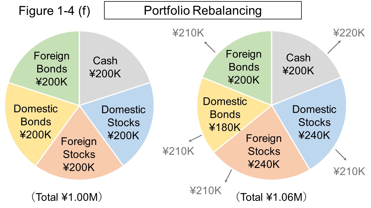
A method called additional rebalancing is also known.
Additional rebalancing is a way of balancing by buying a lower ratio of assets to the target ratio, rather than selling some.
This method provides a compound interest effect while reducing tax payments, as assets with a positive valuation are not sold.
The red line in Figure 1-4 (g) below shows the change in asset value when an additional 50,000 yen had been invested monthly on the Nikkei Stock Average from January 2005 to December 2021.
Also, the cahnge of the Nikkei Stock Average at the end of the year during that period is shown by the blue line, and the change in asset value that similar additional investing was started in January 2008 is shown by the green line.
Since it is not possible to invest directly on the Nikkei Stock Average, Figure 1-4 (g) is just fiction, but similar outcomes should be obtained by using investment trusts and ETFs.
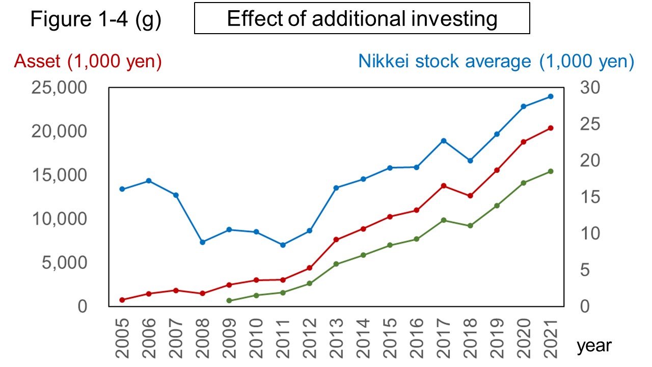
From Figure 1-4 (g), it can be seen that the Nikkei Stock Average fell sharply from 2006 to 2008, but the asset value was not significantly affected.
The reason is that, of course, there was a loss, but since the investment was small at the beginning, the additional amount compensated for the loss.
In addition, even if investing is started at the bottom of the market from January 2009, the asset value shown by the green line will not exceed the asset value shown by the red line.
Table 4 shows the total investment in these two cases and the assets at the end of 2021.
It can be seen that investment started in 2009 has a higher annualized ROI than investment started in 2005, but the final asset value is lower.
This shows that guessing the bottom of the market correctly does not always make a lot of profit.
| Start year | Total investment | Asset at the end of 2021 | ROI | annualized ROI |
| 2005 | 10.2 million yen | 20.4 million yen | 99.8% | 4.4% |
| 2009 | 7.8 million yen | 15.4 million yen | 97.8% | 5.8% |
If you continue to invest, you will be able to receive benefit from the total investment when the market rises.
And if you don't know whether the market will go up or down, it's advantageous to start investing early.
This is because the expected value of investment is showing an upward trend of asset value in the first place.
Also, in the case of Figure 1-4 (g), in addition to the asset value, you can take dividend income not shown in the figure.
The profit from the +10% rate of return and the loss from the −10% rate of return are the same the first time, but the amount will be different if the same rate of return is repeated.
Figure 1-4 (h) shows the change of assets when 1 million yen continues to increase or decrease by 10% every year.
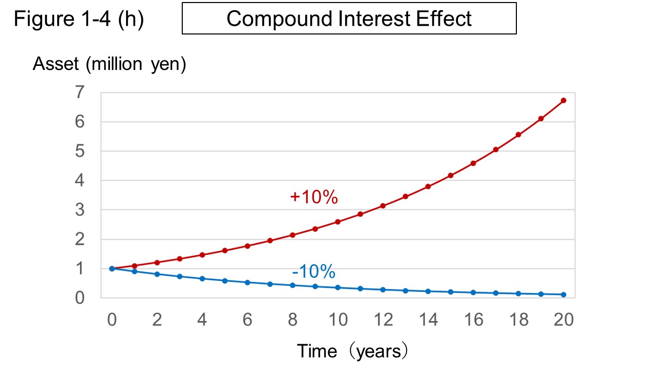
Twenty years later, the asset value of 1 million yen will be about 6.73 million yen if it continues to increase by 10% every year, but it will be about 120,000 yen if it continues to decrease by 10% every year.
The reason for the difference between the increase and the decrease is that if the 10% increase is repeated twice, it will increase by 21%, but if the 10% decrease is repeated twice, it will decrease by only 19%.
Such an effect is called the effects of compounding.
ref 2
The term compound interest is commonly used when assets increase, but this website uses the same term even when assets decrease.
The compound interest effect shows that profits are not limited, but losses are limited to principal, in usual asset management.
The effects of compounding may seem great at first glance, but unless asset value is constantly increasing, such the good luck of the red line in Figure 1-4 (h) won't be come.
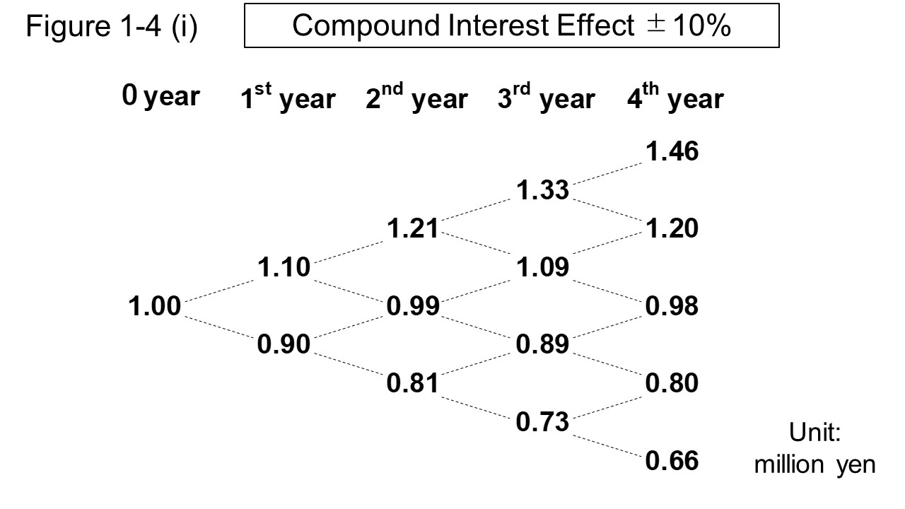
Figure 1-4 (i) shows a simulation in which the value of an asset of 1 million yen is repeatedly increased or decreased by 10%.
In this case, it can be seen that a single loss will return the asset value to about two years ago.
In addition, if the same rate of profit and loss is repeated same times, the asset value will be a slight loss rather than an equal.
As long as the same rate of change continues, the effects of compounding can be considered more general.
Figure 1-4 (j) shows a diagram when the principal P repeats the increase / decrease rate of ±\(r\)%.
In the figure, changes of +\(r\)% are represented by \(r_{+}\), and changes of −\(r\)% are represented by \(r_{-}\).
As \(r_{+}\) continues, the asset value changes to the upper right with the passage of years, and as \(r_{-}\) continues, the asset value moves to the lower right with the passage of years.
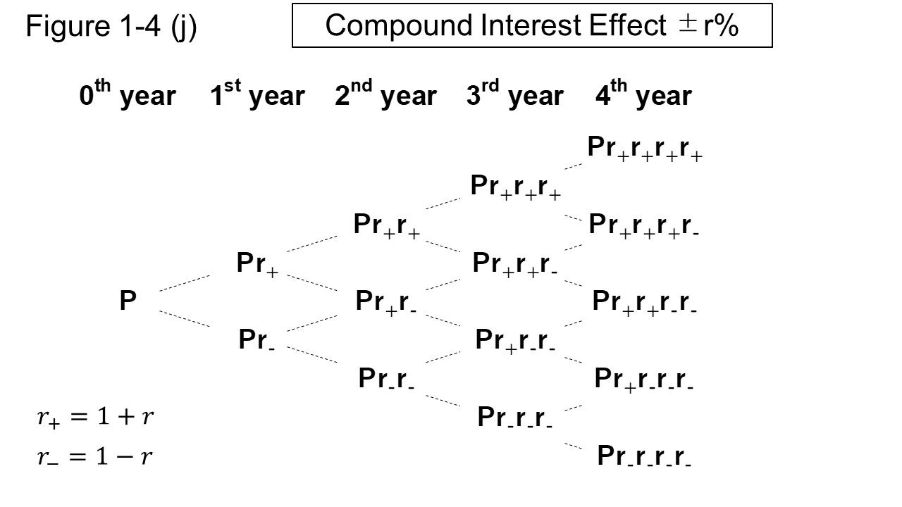
As \(r_{+}\) accumulates, the effect of compounding accelerates asset growth.
However, once \(r_{-}\) is attached, it can be seen that the loss rate affects all the asset values that have increased so far.
And, the reason why the loss occurs when the same increase / decrease rate is repeated same times is that the amount of \(r^{2}\) in the following formula is reduced.
However, this does not mean that the investment is a disadvantageous game.
The diagram in Figure 1-4 (j) shows, to be precise, the forcast of the outcome when the profit is bet additionally on gamble which has a 50% chance of winning or losing and the same rate of increase or decrease.
As already mentioned, investment is a game that has a positive expected value and is expected to have a bottom-up effect on the win rate or increase / decrease rate.
In addition, investors do not need to add profits to same asset.
Therefore, if you manage own assets adequately, investing is a game with no cap on profits, not a game such as you loses all assets.